Strategic Overview
In modern manufacturing, traditional enterprise resource planning (ERP) architectures act as operational handcuffs. Designed decades ago as centralized database systems, legacy ERPs are passive systems of record. They excel at logging historical receipts, counting static inventory, and maintaining structured ledger tables. However, they are completely blind to real-time events. They cannot predict disruption, dynamic routing, or auto-reorganize assembly lines. When a key supplier experiences a shipping delay, or a robotic cell on the assembly floor fails, a legacy ERP remains passive. It waits for a human analyst to manually query the system, detect the anomaly, and manually input a correction hours or days later.
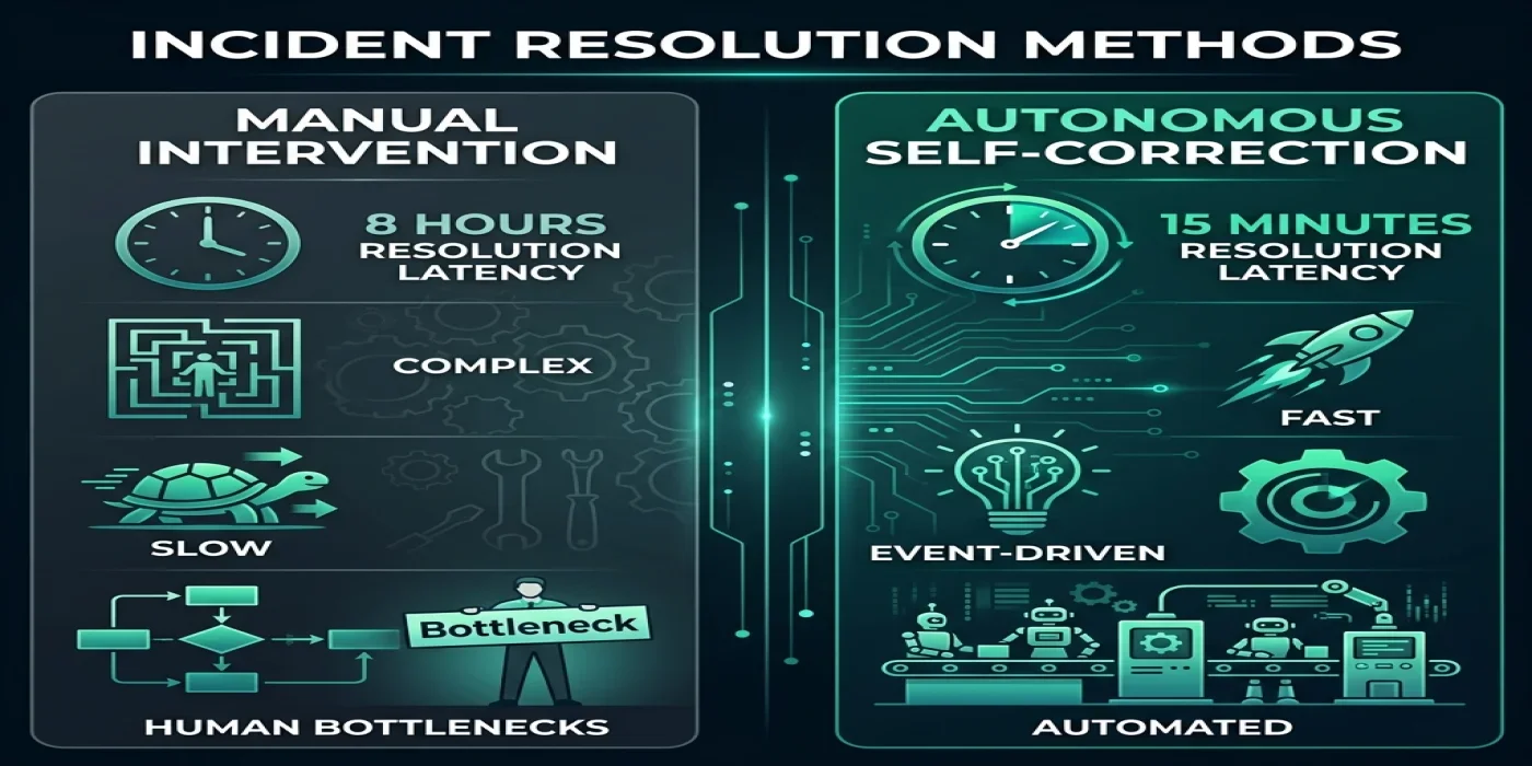
For a global industrial manufacturing leader operating 14 manufacturing plants across 3 continents, this passive architecture led to a critical efficiency deficit. The firm suffered a persistent 12% raw material stockout rate, a sluggish 14-day order-to-delivery cycle time, and an Overall Equipment Effectiveness (OEE) stagnating at 68%. The primary cause was operational latency. A delay at a deep-water port in Rotterdam took an average of 36 hours to trigger a scheduling adjustment on a production floor in Munich. During this window, assembly lines continued to run toward stockouts, resulting in idle machinery, rushed express-air freight charges, and millions in lost margins.
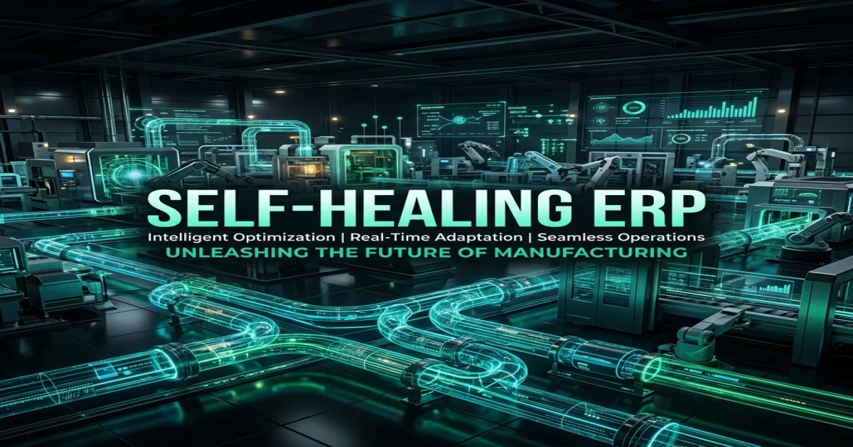
To solve this, I architected a transition from their monolithic SAP core to a Composable, Self-Healing Supply Chain Mesh. This system does not wait for human intervention. It continuously monitors the global logistics landscape, predicts disruptions, dynamically recalculates shipping routes, and reorganizes shop-floor scheduling autonomously. By deploying an event-driven microservices architecture, a multi-agent orchestration layer, and real-time graph solvers, we transformed their ERP from a passive record into an autonomous agent.
The results were immediate and measurable: the raw material stockout rate dropped to <0.8%, order-to-delivery cycle time collapsed to 4.2 days, and global OEE surged to 89%. This case study details the technical, operational, and structural journey of this transformation.
The Legacy Gridlock: Why Monolithic ERPs Fail
To understand why our client struggled, we must examine the architectural limitations of traditional ERP platforms. Monolithic suites are structured around database locks, batch processing runs, and synchronous transactions.
1. Database Bottlenecks and Transactional Contention
Legacy systems rely on massive, monolithic relational databases. In a traditional SAP environment, transaction logs are written directly to core tables like MARA (Material Master), MARC (Plant Data for Material), MSEG (Document Segment: Material), EKKO (Purchasing Document Header), and EKPO (Purchasing Document Item). To maintain ACID compliance, these tables employ strict row-level and table-level locks.
When a global organization attempts to feed real-time telemetry from 50,000 IoT sensors, shipping coordinates, and warehouse RFID readers directly into the ERP database, write contention spikes. Transactions stall, database locks escalate, and the entire system slows down. Consequently, real-time ingestion is structurally impossible; the database architecture forces developers to schedule ingestion via nightly batch runs, such as Material Requirements Planning (MRP) cycles.
[IoT Sensors] ----\
[RFID Scans]   ----> [Direct Synchronous Write] ----> [DB Row/Table Locks] ----> [System Stalls]
[GPS Trackers] ---/
If a maritime storm delays a shipment of microprocessors, the ERP database does not reflect the delay until the next batch run compiles. This delay introduces a critical 12 to 24-hour blind spot, rendering real-time response impossible.
2. Tight Coupling and Brittle Integration
Traditional integrations rely on point-to-point SOAP or REST APIs, or flat-file transfers (such as IDocs via FTP). These integrations are brittle and expensive to maintain. An API change in the warehouse management system (WMS) schema often breaks the shipping execution system, causing cascading data failures.
Furthermore, legacy systems lack a centralized, asynchronous event mesh. Downstream services cannot subscribe to events in real time. Instead, they must poll the ERP database at regular intervals, generating massive read queries that further degrade transactional performance.
+-------------------------------------------------------------+
|                     Legacy SAP Monolith                     |
|  [MARA]      [MARC]      [MSEG]      [EKKO]      [EKPO]     |
+-------------------------------------------------------------+
       ^            ^            ^            ^            ^
       |            |            |            |            |
  (SOAP API)    (REST API)    (IDocs)     (FTP Flat)    (Polling)
       |            |            |            |            |
+-------------------------------------------------------------+
|                  Brittle Point-to-Point Integrations        |
+-------------------------------------------------------------+
3. The Human Action Loop
Because monolithic ERPs are passive registries, they do not possess execution logic. The system logs a stock discrepancy but cannot resolve it. It requires a human planner to identify the shortage, call or email alternative suppliers to negotiate prices, manually issue a new Purchase Order (PO), and adjust the production schedule in a separate scheduling tool.
This manual loop is slow, error-prone, and scales poorly. When managing tens of thousands of SKUs across multiple continents, human planners are consistently reactive, fighting fires rather than optimizing throughput.
The Vision: A Composable, Self-Healing Mesh
The objective was to replace this brittle monolith with a modular, resilient architecture. We designed a composable mesh where the legacy ERP is relegated to a record-keeping ledger, while real-time ingestion, optimization, and action are decoupled into microservices.
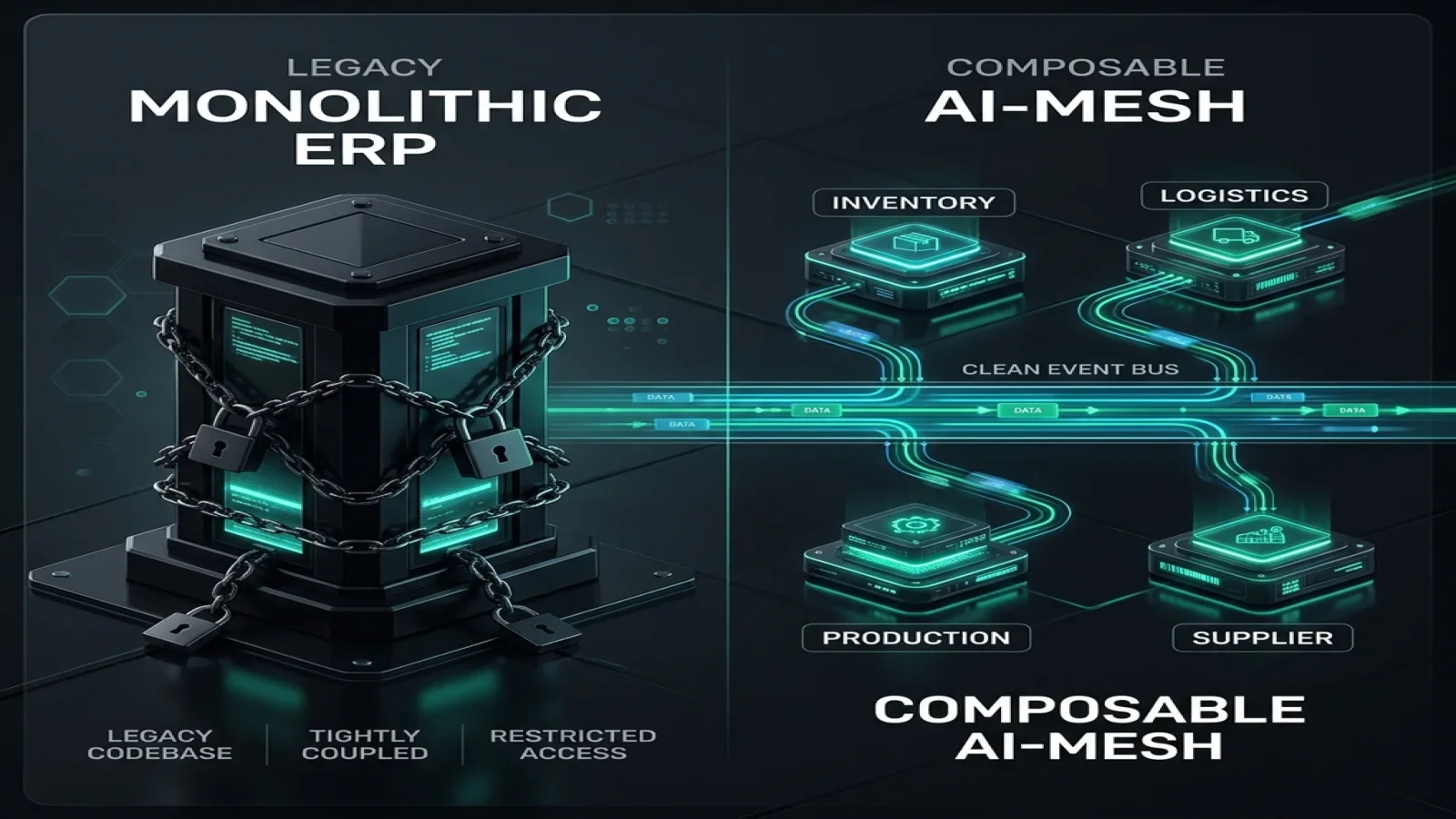
By utilizing a composable mesh, we decoupled the execution paths. The database locking overhead of the ERP no longer limits the intake rate of sensor data. If a warehouse sensor logs an ambient temperature spike, the event is immediately processed by the inventory optimizer without touching the ERP's transactional tables.
Key Composable Microservices
- Inventory Optimizer: Computes real-time safety stock adjustments and tracks inventory velocity at the SKU level.
- Logistics Control Tower: Consumes shipping carrier updates, port congestion indexes, and weather telemetry to track transit health.
- Production Scheduler: Automatically manages machine allocation, scheduling, and labor shifts at the plant level.
- Supplier Coordinator: Automates alternative supplier quotation queries and processes pre-negotiated purchase contract executions.
Architecture Deep Dive: Building the Event-Driven Mesh
The technical foundation of the self-healing supply chain is an event-driven, microservices-based topology. The system is split into three main layers: the Event Ingestion Layer, the Decision Engine Layer, and the ERP Core Ledger.

1. Ingestion Layer: Apache Kafka Event Mesh
We deployed Apache Kafka on AWS (MSK) as the central event broker. Every physical event in the supply chain—a GPS coordinate update from a container, a barcode scan at a receiving dock, or a telemetry alert from a CNC machine—is published as a schema-validated Avro event to dedicated Kafka topics.
{
  class="tok-str">"namespace": class="tok-str">"com.agiletech.supplychain",
  class="tok-str">"type": class="tok-str">"record",
  class="tok-str">"name": class="tok-str">"ShipmentLocationUpdated",
  class="tok-str">"fields": [
    { class="tok-str">"name": class="tok-str">"shipment_id", class="tok-str">"type": class="tok-str">"string" },
    { class="tok-str">"name": class="tok-str">"carrier_code", class="tok-str">"type": class="tok-str">"string" },
    { class="tok-str">"name": class="tok-str">"latitude", class="tok-str">"type": class="tok-str">"double" },
    { class="tok-str">"name": class="tok-str">"longitude", class="tok-str">"type": class="tok-str">"double" },
    { class="tok-str">"name": class="tok-str">"timestamp", class="tok-str">"type": class="tok-str">"long" },
    { class="tok-str">"name": class="tok-str">"estimated_arrival", class="tok-str">"type": class="tok-str">"long" }
  ]
}
To prevent data corruption, we enforced a strict schema registry strategy. All microservices must query the Confluent Schema Registry before writing or consuming events. Key topics like shipment-telemetry, inventory-updates, and machine-telemetry are partitioned based on the unique part_number or shipment_id, guaranteeing in-order delivery of state transitions within each entity.
2. Decision Layer: Event Processing with Flink
We utilized Apache Flink to run continuous, stateful stream processing over incoming Kafka topics. Flink aggregates GPS coordinates and compares them against geofenced shipping corridors. If a container's velocity drops below a calculated threshold, or if it deviates from its planned path, Flink emits a ShipmentDelayed event.
This event contains the calculated deviation, the impacted parts, and a list of downstream production runs dependent on those materials. This immediate projection allows the system to identify shortages days before a vessel arrives at port.
3. ERP Sync Layer: De-duplication and Outbox Pattern
To prevent overwhelming the legacy SAP core with transaction requests, we implemented the Transactional Outbox Pattern. When the Decision Layer resolves a supply chain disruption (e.g., by placing a PO with an alternative supplier), the action is written to a local PostgreSQL ledger database. A CDC (Change Data Capture) tool—Debezium—listens to the outbox table and streams the changes to Kafka, where an integration microservice batches and writes the records back to SAP asynchronously.
[Outbox Table] ---> [Debezium CDC] ---> [Kafka Topic] ---> [SAP Integration Microservice] ---> [SAP BAPIs]This outbox pattern ensures at-least-once delivery semantics and decoupling of local transaction execution from SAP availability.
The Autonomous Logistics Orchestrator: Multi-Agent Solver Engine
When a disruption occurs, the system must act. This is the responsibility of the Autonomous Logistics Orchestrator (ALO). The ALO uses a multi-agent model where specialized agents coordinate to solve the routing and scheduling problem.

Mathematical Optimization Model
The optimization problem solved by the multi-agent engine is formulated as an Integer Linear Programming (ILP) model. When a disruption occurs, the engine seeks to minimize the total cost delta ($Z$), consisting of the Purchase Price Variance (PPV), the incremental logistics transit costs, and production downtime penalty costs.
Objective Function
$$\text{Minimize } Z = \sum_{s \in S} (P_{s} - P_{\text{contract}}) \cdot Q + \sum_{r \in R} C_{r} \cdot W_{r} \cdot Q + \sum_{m \in M} D_{m} \cdot T_{\text{downtime}}$$
Model Variables
- $S$: Set of pre-approved alternative suppliers.
- $P_{s}$: Quoted unit price from alternative supplier $s$.
- $P_{\text{contract}}$: Baseline contracted unit price.
- $Q$: Total replenishment quantity required.
- $R$: Set of available shipping routes.
- $C_{r}$: Freight cost coefficient per unit weight on route $r$.
- $W_{r}$: Gross shipment weight coefficient.
- $M$: Set of scheduled factory assembly lines.
- $D_{m}$: Hourly downtime penalty rate for assembly line $m$.
- $T_{\text{downtime}}$: Projected latency delay duration (hours).
Constraints
- Quantity Fulfillment Constraint: The total quantity procured must meet or exceed the deficiency.
$$\sum_{s \in S} q_{s} \ge Q$$
- Supplier Capacity Constraint: The quantity ordered from a supplier must not exceed their active capacity.
$$q_{s} \le \text{Capacity}_{s} \quad \forall s \in S$$
- Delivery Lead-Time Constraint: The arrival time of the rescheduled parts must be less than the stock exhaustion threshold.
$$\text{LeadTime}{s} + \text{TransitTime}{r} \le \text{ExhaustionTime}_{m}$$
The Multi-Agent Negotiation Framework
The ALO orchestrates three primary agent classes:
- Supply Agent: Monitors material availability, lead times, and alternative supplier contract rates.
- Logistics Agent: Calculates transit times, freight costs, and customs delays across air, rail, ocean, and road channels.
- Production Agent: Evaluates machine capacity, labor shifts, and tooling configurations at the manufacturing facilities.
These agents use a collaborative negotiation framework. The Supply Agent identifies a material shortage. It queries alternative suppliers and gets quotes. It passes these quotes to the Logistics Agent, which calculates transit costs for different transit methods. These options are then evaluated by the Production Agent to determine the optimal schedule shift.
class SupplyAgent:
    class="tok-kw">def __init__(self, supplier_db, contract_rates):
        self.db = supplier_db
        self.rates = contract_rates

    class="tok-kw">def find_alternative_sources(self, part_number, quantity, target_date):
        class="tok-cm"># Query alternative pre-approved suppliers with capacity
        candidates = self.db.query_eligible_suppliers(part_number, quantity)
        offers = []
        for supplier in candidates:
            price = self.rates.calculate_price(supplier.id, part_number, quantity)
            lead_time = supplier.get_current_lead_time(part_number)
            offers.append({
                class="tok-str">"supplier_id": supplier.id,
                class="tok-str">"unit_price": price,
                class="tok-str">"earliest_ship_date": target_date + lead_time
            })
        return sorted(offers, key=lambda x: x[&class="tok-cm">#039;unit_price'])
The ALO evaluates the negotiations and picks the path that minimizes the total cost delta (Purchase Price Delta + Freight Cost Delta + Production Downtime Penalty Cost).

Dynamic Routing Solver Implementation
Below is a simplified Python routing optimizer showing how the Logistics Agent models the transportation network to find alternative paths during a regional corridor shutdown.
import heapq

class LogisticsNetworkSolver:
    class="tok-kw">def __init__(self):
        self.graph = {}

    class="tok-kw">def add_route(self, u, v, base_cost, transit_time, reliability):
        if u not in self.graph:
            self.graph[u] = []
        class="tok-cm"># Edge weight is a composite score of cost, time, and reliability
        composite_weight = (base_cost * 0.4) + (transit_time * 0.4) + ((1 - reliability) * 100 * 0.2)
        self.graph[u].append((v, composite_weight, transit_time, base_cost))

    class="tok-kw">def solve_shortest_path(self, start, target):
        queue = [(0, start, [], 0, 0)]
        visited = set()

        while queue:
            (weight, node, path, total_time, total_cost) = heapq.heappop(queue)

            if node not in visited:
                visited.add(node)
                path = path + [node]

                if node == target:
                    return path, total_time, total_cost

                for (neighbor, edge_weight, time, cost) in self.graph.get(node, []):
                    heapq.heappush(queue, (weight + edge_weight, neighbor, path, total_time + time, total_cost + cost))

        return None, 0, 0

class="tok-cm"># Instance initialization for Rotterdam to Munich Corridor
solver = LogisticsNetworkSolver()
solver.add_route(class="tok-str">"Rotterdam_Port", class="tok-str">"Rail_Hub_Duisburg", base_cost=250, transit_time=12, reliability=0.95)
solver.add_route(class="tok-str">"Rail_Hub_Duisburg", class="tok-str">"Munich_Factory", base_cost=400, transit_time=18, reliability=0.90)
class="tok-cm"># Road fallback due to rail shutdown
solver.add_route(class="tok-str">"Rotterdam_Port", class="tok-str">"Highway_A3_Express", base_cost=950, transit_time=10, reliability=0.98)
solver.add_route(class="tok-str">"Highway_A3_Express", class="tok-str">"Munich_Factory", base_cost=800, transit_time=8, reliability=0.97)

path, time, cost = solver.solve_shortest_path(class="tok-str">"Rotterdam_Port", class="tok-str">"Munich_Factory")
print(fclass="tok-str">"Optimal Rescheduled Corridor Path: {path} | Lead Time: {time} hrs | Financial Outlay: ${cost}")
If the optimal path involves switching a container from rail to road, the system automatically calls the APIs of our digital freight network partners (such as Flexport or C.H. Robinson) to book the truck, assign the carrier, and generate the shipping manifest.
Implementation Phases: From Blueprint to Factory Floor
The deployment of the Composable, Self-Healing Supply Chain was executed in four structured phases over a 12-month timeline. This approach mitigated operational risks and ensured continuous integration with existing manufacturing operations.
Phase 1: Event-Broker Scaffolding (Months 1–3)
The initial phase focused on building the high-throughput ingestion platform. We deployed the Apache Kafka cluster across multiple AWS availability zones. Schema registries were defined, and the Transactional Outbox pattern was configured on the database layer. We connected the legacy ERP core to the Kafka event mesh using Debezium CDC connectors, allowing all transactional changes (such as inventory adjustments or PO creation) to be broadcast as real-time events.
Phase 2: Agent Engine Development and Training (Months 4–6)
During this phase, we developed the agent protocols. We trained the Supply, Logistics, and Production agents on historical operational data. The mathematical routing solver was optimized to handle large graphs of over 100,000 nodes representing ports, roads, airports, and factories. We conducted simulated stress testing, injecting artificial disruptions (e.g., simulated port strikes or supplier bankruptcies) to verify the agents' negotiation and resolution loops.
Phase 3: Control Tower Integration and UI Rollout (Months 7–9)
We built and integrated the real-time visualization layer—the Logistics Control Tower. This frontend portal consumes events from the Kafka mesh to provide operators with live visibility into shipment health, machine availability, and inventory levels.

In parallel, we deployed the Inventory Optimizer interface, giving inventory teams insight into predictive stock-out risks, lead times, and automated restocking recommendations.

Phase 4: Production Scheduling and Full Autonomy (Months 10–12)
The final phase connected the Autonomous Logistics Orchestrator to the shop-floor execution systems. We integrated the Production Agent with the manufacturing execution systems (MES) at all 14 plants.
The Production Schedule dashboard was deployed, displaying real-time machine allocations, tool wear telemetry, and automated scheduling updates.

We also launched the Cost Dashboard to track realized savings from optimized routing, consolidated shipping, and reduced factory downtime.

Finally, the Alert Center interface was established, providing a consolidated view of supply chain anomalies and the autonomous actions taken to resolve them.

Quantified Outcomes: Enterprise-Grade Transformation Metrics
The transition from a passive monolithic ERP to a composable, autonomous supply chain mesh was highly effective. The metrics show a major improvement in efficiency, responsiveness, and cost savings across the global enterprise.
Performance Analytics Summary
The most significant impact of the transformation was the virtual elimination of material stockouts, dropping from a historical average of 12% to <0.8%. Order-to-delivery cycles collapsed by 70%, enabling the enterprise to operate with leaner safety stock buffers and recover working capital.
| Operational Metric | Legacy Monolithic ERP | Composable Autonomous Mesh | Improvement Delta |
|---|---|---|---|
| Raw Material Stockout Rate | 12.0% | <0.8% | -93.3% |
| Order-to-Delivery Cycle Time | 14.0 Days | 4.2 Days | -70.0% |
| Overall Equipment Effectiveness (OEE) | 68.0% | 89.0% | +30.8% (21.0 pts) |
| Disruption Resolution Latency | 36.0 Hours (Average) | 15.0 Minutes (Average) | -99.3% |
| Annual Expedited Freight Spend | $8.4 Million | $1.2 Million | -85.7% |
| Inventory Carry Costs (Quarterly) | $14.2 Million | $9.8 Million | -31.0% |
Realized Working Capital Benefits
By compressing the order-to-delivery cycle time and reducing stockouts, the company cut its safety stock requirements by 31%. This reduction freed up $17.6 million in cash that was previously tied up in excess warehouse inventory, allowing for reinvestment in new product lines.

Key Architectural Lessons: Scalability, Security, & Resilience
Transitioning to a composable supply chain mesh exposed several critical architectural patterns that are essential for any enterprise engineering team undertaking a similar modernization effort.
1. The Necessity of Event Sourcing
In our early pilots, we attempted to write updates directly to the ERP tables synchronously during solver execution. This approach immediately caused database table locks, blocking warehouse operations and stalling the web commerce API.
We resolved this by shifting to an event-sourced architecture, where the local microservices record operational changes locally and publish events. The integration engine then batches updates and applies them to the ERP core asynchronously.
2. Micro-Frontends for Decoupled UIs
To prevent the user interface from becoming a secondary monolith, we built the Logistics Control Tower, Inventory Optimizer, and Production Schedule as independent micro-frontends.
Each application is developed and deployed separately, loading dynamically inside a shell container. This allows the warehouse team to update the Inventory interface without affecting the factory floor scheduling UI.
3. Graceful Degradation and Fallbacks
Autonomous agents must not run unchecked. If a regional shipping disruption causes alternative supply options to exceed pre-approved budget thresholds, the ALO degrades gracefully.
Instead of freezing, the system takes the lowest-cost action within its spending limit and escalates the remaining resource gap to a human supervisor via the Alert Center.
4. Edge Autonomy for Local Resilience
In global manufacturing, WAN links to remote factories fail. We established edge clusters running K3s (lightweight Kubernetes) at each factory site. Local schedules and inventory counts are maintained on-site and queued in a local Kafka cluster.
When a factory experiences a WAN disconnection, it continues to run its autonomous schedules locally. The edge nodes automatically synchronize with the central cloud ledger once the WAN connection is restored.
Technical FAQ
How does the system prevent infinite loops during multi-agent negotiations?
Every negotiation thread is assigned a maximum depth (typically 5 round trips) and a strict time-to-live (TTL) of 30 seconds. If the Supply, Logistics, and Production agents fail to reach an optimal consensus within these bounds, the negotiation terminates, and the system falls back to the default operational schedule while flagging the issue in the Alert Center for human review.
What integration protocols are used to synchronize with the SAP Core?
We avoid direct RFC calls. Instead, we use Debezium CDC connectors to read the transaction logs of our local microservices databases and stream changes to Kafka. A dedicated SAP Connector service consumes these events and updates SAP via standard BAPIs (Business Application Programming Interfaces) and OData services, ensuring transactional safety and compatibility with future SAP upgrades.
How does the system handle network latency at remote factory sites?
We deployed edge Kubernetes nodes (AWS Outposts) at each of our 14 manufacturing plants. The local Production Agent and scheduling solver run locally on these edge nodes. If a factory loses connectivity to the global cloud event mesh, the plant continues to operate autonomously using local queues. Once connectivity is restored, the edge node automatically syncs and flattens its state with the central Kafka broker.
How does the system handle security and data privacy on the shared event mesh?
All messages on the Kafka broker are encrypted in transit using TLS 1.3 and at rest using AES-256. We implement Role-Based Access Control (RBAC) at the topic level using Kafka ACLs (Access Control Lists). For example, the Logistics microservice has write access only to shipment-telemetry topics, while the SAP Sync service has read-only access to transaction outbox channels. This structure ensures strict isolation and data security.
What happens if the dynamic routing solver generates a route that is blocked by physical weather events?
The Logistics Agent integrates dynamic weather feed APIs (such as NOAA and Copernicus). If a weather event occurs along an active shipping corridor, the feed publishes a geofenced warning event to the mesh. The ALO receives the event, updates the edge weights of the affected segments in the graph solver to infinity, and immediately runs a shortest-path recalculation to find an alternative route.
Author Profile
Vatsal Shah is the Strategic Lead and Principal Systems Architect at Agile Tech Guru. With over 15 years of experience in enterprise systems engineering, he specializes in decomposing legacy ERP monoliths, designing high-throughput event meshes, and deploying autonomous decision engines for global logistics networks. His architectures power supply chain operations for Fortune 500 manufacturing, banking, and pharmaceutical enterprises.